Equation of the Day #17: Confounding Compounding Interest

Eons ago in math class, I was taught the math behind compound interest. It’s an interesting problem with real world applications in financial investment; eventually, my class was shown an expression that looks like this,

and asked what this expression approaches when N → ∞. (I will set up the expression in a bit.) Naively, I expected that, since N becomes large, 1/N must be really small, so the inside of the parentheses approaches 1. Since 1 to any power is 1, it made sense to me that this expression approaches 1 as N becomes really large. But if you take your calculator and plug in values, you will find that this isn’t the case. In fact, for N = 1000, you get that

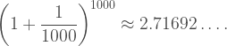
Definitely not 1. In fact, this expression approaches a number which is widely recognized in mathematics today:

Why is this? What does the strange expression at the top have to do with base of the natural logarithm? My teenage self was utterly confused by this, and I wouldn’t be honest if I said this oddity hasn’t nagged at the back of my head since then. The reason for this confusion, I think, is because I’ve only ever looked at this problem as pure numbers – the expression I started with – but there is another way to see it. By the end of this article, I hope I can convince you that there is no way that the expression at the top could possibly be 1, and in fact must be the number e.

Let’s consider the problem of compound interest. Say you decide to invest $1 into an account which, after one year elapses, an incredibly generous bank gives you an interest rate of 100% of the dollar you invested. Thus, after one year you end up with a total value of $2. If you had instead invested $5, you would end up with $10 after one year, and so on. If we call the principal investment P, then the total amount of money you have after one year is 2P. So far, so good. But in reality, investment percentages are much lower. Say instead of a 100% interest rate, you have an interest rate of 5%. After one year elapsed, your $1 will have accrued interest equal to 5% of that dollar, or 5 cents. So, after one year, your total amount of money from your investment is $1.05. Instead of turning $1 into $2, you’ve turned 20 nickels into 21 nickels. This return is not as good, so you want to get as high an interest rate as possible. To be more general, we’ll call the percentage rate x. If you invest P dollars as principal, after one year you end up with your principal, P, plus the interest accrued, which is x times P. As a mathematical expression, this would be (1+x)P. Perhaps you might see a hint of things to come here.

Nothing I’ve said is particularly groundbreaking, so let’s spice things up a bit. Now let’s say the bank offers not just to apply interest to your account after one year but to apply interest halfway through the year as well. Your annual interest rate is still x, but this rate is divided up twice throughout the year. So, after half a year, you end up with your principal plus half the interest you would have had at the end of the year; in other words, you end up with your principal, P, and an interest of x/2 times P. A little algebraic manipulation gives

Then, at the end of the full year, you end up with the money you had halfway through the year, (1 + x/2)P, plus the interest accrued on this money value, (x/2)(1 + x/2)P. The result, after some algebraic manipulation, is

Let’s think of this in terms of our $1 principal at 100% interest. (We’ll tack the principal P back on at the end.) After half a year, you end up with $1.50, since half the interest rate is applied to the principal. After the full year, you end up with $2.25, or $1.50 plus half of $1.50 (75 cents). As a savvy investor, you realize that applying interest more often also nets you more cash, so you try to get the bank to compound its interest not just semiannually, but quarterly. The trend is much the same, and at the end of the year, with interest compounded four times, your $1 at 100% interest ends up being $2.44. For a general interest rate of x, your principal investment P becomes (1 + x/4)⁴P.

This is the origin of the first expression. If N is the number of times the interest is compounded, and the interest rate is 100% (x = 1), we get the expression I showed at the beginning. Plugging in numbers reveals to us that the return on investment indeed goes up, but it’s not clear from looking at the expression why it does so. So, let’s move away from the expression and instead view it by graphing the curve it describes.

First, let’s look at N = 1, or the relationship y = (1 + x/1)¹.

Remember, the x-axis represents the percent interest applied to the principal. This graph is a line with slope 1, shifted from the center one unit. The shift is either up or to the left depending on which direction you prefer. As we’ll see shortly, I want to consider it a shift to the left by one unit.

Let’s increment the compounding frequency from N = 1 to 2. How does our return after one year look?

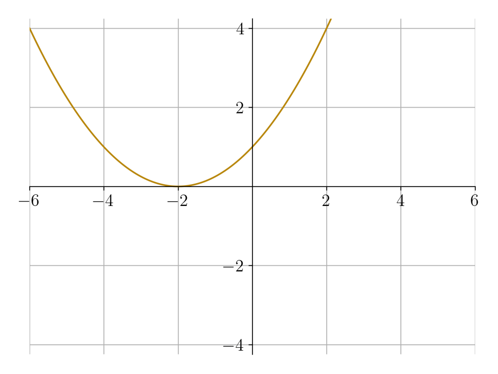
The equation is y = (1 + x/2)². This, then, is a quadratic equation, so the shape above is a parabola. It curves upward, since the coefficient on x is positive. This parabola is also shifted, since its vertex is not at the origin, and this time the shift is clearly to the left by two units. To recap, the N = 1 curve was a degree 1 polynomial shifted to the left by 1, and the N = 2 curve was a degree 2 polynomial shifted to the left by 2. Will this pattern hold for N = 3?

It seems so! This is a cubic function (degree 3), shifted to the left by 3. In fact, if we rearrange the original expression for compounded interest, we can glean this fact.

The final expression is the one we want chew on for a bit. What f(x + N) means is that we have an unshifted function, called f, whose input (x) has been increased by N units. This results in a shift of the output of f to the left by N units.

Why to the left? By increasing the input by a set amount, the function looks ahead in the input space. By looking ahead, a lower x value receives an output that should occur later, resulting in a leftward shift.

The purple function peaks before the gold function, since its inputs look ahead three units.
The value of the gold function at x = 0 occurs in the purple function at x = −3.

What is the unshifted function f(x) for this problem? It’s a polynomial of degree N with only one term (x^N) scaled down by the factor N^N,

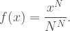
Taking all of this together, we get this equation.

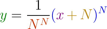
In words, the curve describing the money accrued after one year with a principal of $1 compounded N times at x percent interest is a polynomial of degree N shifted to the left by N units and scaled so that when x = 0, y = 1.^[1]

The last statement is actually more obvious when the equation is in its original form, but you can check it easily enough by plugging in x = 0. The point (0, 1) is a fixed point when we vary N, and this is actually critical to understanding the limiting behavior of this function as N approaches infinity. As we compound the interest more times per year, the accrued value is described by an ever higher-degree polynomial function appropriately shifted and scaled to pass through (0, 1). In fact, forcing the curve through the point (0, 1) is the mathematical way of saying that an interest rate of 0% returns your principal ($1) with zero interest after one year, which is what should happen.

But let’s not get too far away from our goal: we want to know what happens when N gets really big. Let’s see what the function looks like when, say, N = 100.

That looks very similar to the elementary function exp(x). In fact, we can prove that in the limit N → ∞, the two functions are equal. What defines the function exp(x) is that

1. The derivative of exp(x) is itself.
2. exp(0) = 1.

Condition 2 is already met by our function y for all N. The condition left to prove, then, is that dy/dx = y in the limit N → ∞. Since y is just a polynomial, this is straightforward.

The key step is noticing that N − 1 approaches N in the limit as N → ∞, hence the jump between the third- and second-to-last lines. So there we have it; if y describes money accrued after one year compounded N times at a rate of x percent, then y becomes exponential growth for continuously compounded interest (as N → ∞).

And now we can address the limit that kicked off this article. By framing this problem with variable interest rate (x), we get an expression describing a polynomial curve instead of a single number for a single interest rate (100%). The limiting behavior of the value obtained at x = 1 simply falls out of the behavior of the curve rather than arising from some black magic number nonsense. Since we’re talking about a family of polynomials, shifted left by a number of units equal to the degree of the polynomial and scaled to always pass through the point (0, 1), such a curve can only simplify to a value of 1 when the degree is zero, and taking the limit as the degree becomes as large as possible means that we can abandon the idea that y could equal 1 at any other input on the curve.

Actually taking the limit at x = 1 yields exp(1) = e, no confusion necessary.

Additionally, this framing of the problem illustrates a known property of exponential growth, namely that exp(x) grows faster than any polynomial. The reason is clear: exp(x) is the limit of taking a specific polynomial to infinite degree. It’s not even something we have to prove; it just falls out of the limit. I think that’s wonderful.

(Made in Manim.)

This is also an excellent reminder that exp(x) is special, not the base e. In fact, putting e on a pedestal is what leads to the opening equation being taught in math class (and thus the introduction of confusion to the student) instead of the more intuitive expression involving a variable input x.

Finally, I want to address the fact that the expression for y only touches on how much money is accrued after a single year while varying the interest rate, x. If instead we wanted to frame this as the amount of money accrued after t time with an interest rate r, we would just replace x with the product rt. If t is measured in years, r is the annual interest rate. With this shift in variables, N now represents the total number of times the interest was compounded over the entire time period t. In that case, we still end up with the same expressions, just with the horizontal axis scaled by the rate factor r, and we get the good old formula^[2]

for continuously compounded interest.

Footnotes

1. Shoutout to Kalid Azad at Better Explained for this kind of explanation.

2. Not to be confused with shampoo.